Target Categories in CASP8
Some targets are easy to predict, as they have very close templates among known structures, other targets are quite challenging. It is essential to evaluate predictions taking into account target difficulty, since performance of different algorithms depends on it. Grouping targets into categories of approximately the same prediction difficulty brings out the flavors of how each method deals with different target types.
In the early days of CASP, targets were classified in three general categories: comparative modeling, fold recognition and ab initio prediction, to reflect the method that was used to obtain models. It became clear with time that the best approach is to use a combination of various methods as what matters is the quality of the final prediction. Therefore, it is logical to group targets into categories by the prediction quality.
It appears that a general approach described here leads to a well-defined boundaries between categories coming out naturally from the data. The approach is rooted in the suggestion by the Baker group to use prediction scores of the top 10 models (see ROBETTA evaluation pages) and is similar to what we used for target classification in CASP5 assessment 1). We resorted to a traditional model quality metric that stood the test of time – LGA GDT-TS scores. Targets for which domain-based evaluation is essential, as established by our analysis, were split into domains, and other targets remained as whole chains and were considered as single domain targets for evaluation purpose. This procedure resulted in 147 "domains" gathered from 125 targets. For each of these domains, top 10 GDT-TS scores for the first server models were averaged and used as a measure of each target's difficulty.
We looked for naturally emerging clusters in these average GDT-TS scores and used density-based algorithm. Gaussian kernel density estimator is a function
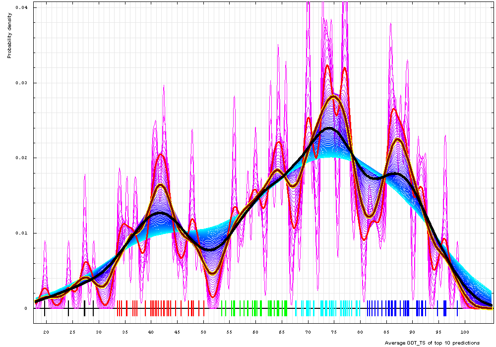
We plotted estimated densities for varying bandwidths, from 0.3 to 8.2 GDT-TS % units. Apparently, lower end bandwidth is too small and results in too many clusters (magenta curves on a plot below). Higher bandwidths around 8% (cyan curves) reveal two major clusters: a large cluster centered at about 73% GDT-TS and a smaller one around 41%. These major clusters can be used for evaluation as they demonstrate that the dataset splits naturally into two groups: "hard" and "easy", with 52% GDT-TS defining a boundary between the groups: surprisingly non-surprising cutoff. Bandwidth of 4% (black curve) yields three groups: hard, medium and easy, with the cutoffs 52% and 81%, i.e. this "medium" group splits from former "easy" group of a two-cluster breakdown. Finally, 2% bandwidth (yellow-framed brown curve) reveals 5 groups, and this is about the right number for evaluation of predictions. GDT-TS bounds between these groups are 30%, 52%, 67% and 81%. We term these categories: FM (free modeling, as predictors are free to do anything they can, they still fail to predict these targets right), FR (fold recognition, to give a tribute to historic category), and CM_H, CM_M, CM_E (comparative modeling – hard, medium and easy). We use these categories to evaluate predictions.

Domains:
Gaussian kernel density estimation of domain GDT-TS scores for the first model GDT-TS
averaged over top 10 servers, plotted at various bandwidths (= standard deviations).
These average GDT-TS scores for domains are shown as a spectrum along the horizontal axis: each bar
represents a domain. The bars are colored according
to the category suggested by this analysis: black - FM; red - FR; green - CM_H; cyan - CM_M; blue - CM_E.
The family of curves with varying bandwidth is shown. Bandwidth varies from 0.3 to 8.2 GDT-TS % units with a step of 0.1, which corresponds to the
color ramp from magenta through blue to cyan. Thicker curves: red, yellow-framed brown and black, correspond to bandwidths 1, 2 and 4 respectively.
Bounds found by the kernel density analysis partition target domains into the following categories.
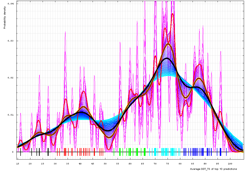
This analysis repeated for the whole chain predictions revealed identical trends, and the same cutoffs of 30%, 52%, 67%, 81% can be used to determine the target category from the top 10 averaged first model GDT_TS scores:

Whole chains:
Gaussian kernel density estimation of whole chain GDT-TS scores for the first model GDT-TS
averaged over top 10 servers, plotted at various bandwidths (= standard deviations).
These average GDT-TS scores for whole chains are shown as a spectrum along the horizontal axis: each bar
represents a target. The bars are colored according
to the category suggested by this analysis: black - FM; red - FR; green - CM_H; cyan - CM_M; blue - CM_E.
The family of curves with varying bandwidth is shown. Bandwidth varies from 0.3 to 8.2 GDT-TS % units with a step of 0.1, which corresponds to the
color ramp from magenta through blue to cyan. Thicker curves: red, yellow-framed brown and black, correspond to bandwidths 1, 2.5 and 4 respectively.
1) L.N.Kinch, J.O.Wrabl, S.S.Krishna, I.Majumdar, R.I.Sadreyev, Y.Qi, J.Pei, H.Cheng, and N.V.Grishin (2003) "CASP5 Assessment of Fold Recognition Target Predictions". Proteins 53(S6): 395-409